Excel表格中单元格的斜线是如何制作出来的？

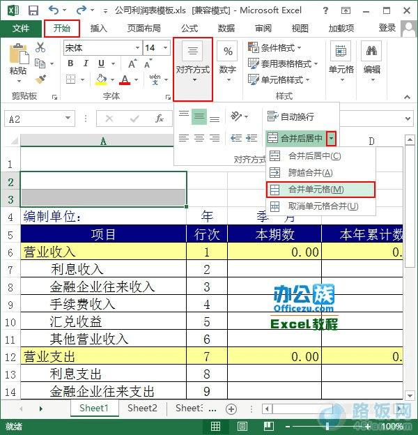
1、 用Excel2013打开一篇表格，选中需要合并的单元格，然后选择“开始”选项卡下的“对齐方式”选项组，并单击“合并后居中”右侧的下拉按钮，选择“合并单元格”选项。

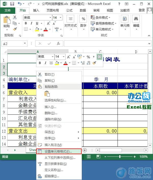
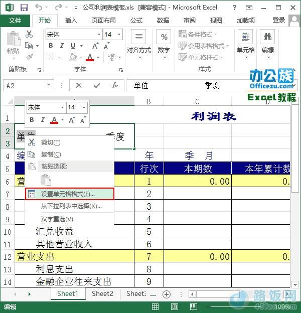
2、 现在我们选中合并的单元格，并单击鼠标右键，在弹出的快捷菜单中选择“设置单元格格式”选项。

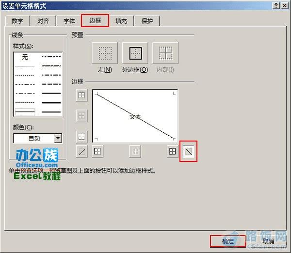
3、 此时会弹出一个“设置单元格格式”对话框，我们切换到“边框”选项卡，并在“边框”栏中选择最右侧的按钮，然后单击“确定”按钮。

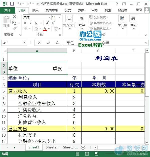
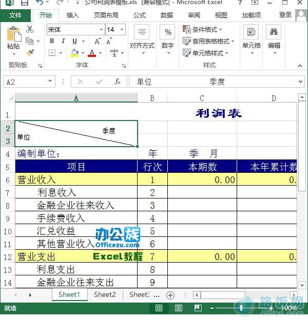
4、 现在边框中已经插入了上述斜线，我们双击单元格，并在其中输入我们需要的内容，注意两个词语分开写在单元格的两边。

5、 我们选中左边的词，并单击鼠标右键，选择“设置单元格格式”选项。此时会弹出一个“设置单元格格式”对话框，我们选择“特殊效果”区域中的“下标”，并单击确定按钮。

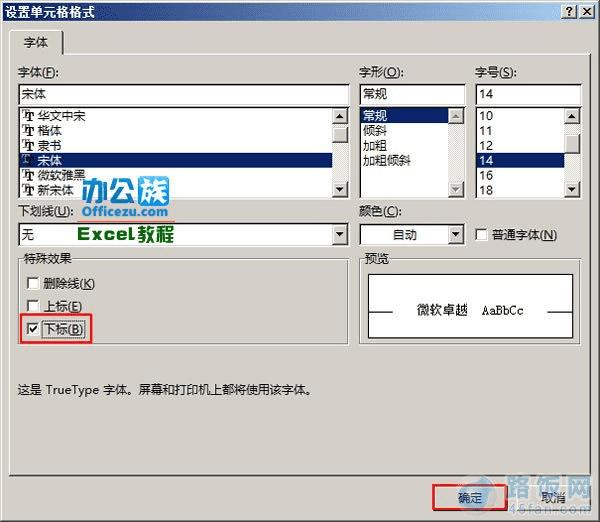
6、 按照同样的方法设置上标，完成之后我们就会看到这样的效果。

提示：大家如果仅需要在某一个单元格中设置上下标，则省略本文中的第1个步骤即可。